EN
 FR
 DE
 IT
 PT
 ES


SigmaPlot: statistical analysis and scientific graphs, 2026 guide
A scientific graph needs to do more than look good in a presentation: it should make clear what was measured, how much the results vary and how far the conclusion can reasonably go. When those details matter, a specialist tool helps you turn a table of numbers into a figure that others can understand and review.
SigmaPlot brings scientific graphing, statistical analysis and curve fitting into a single environment. Its value lies in connecting those tasks: exploring the data, choosing an appropriate analysis and presenting the result without losing sight of the original observations. This guide works through that process using hypothetical numerical examples and practical decisions relevant to laboratory work, engineering, research and teaching.
2026 is the year of this guide; the licence discussed is SigmaPlot 14. These are not two names for the same software version, and this guide does not attribute features introduced in later editions to that licence.
1. What SigmaPlot brings to scientific work
A specialist program becomes useful when you need control over details that affect interpretation: a logarithmic axis, asymmetric error bars, several series on the same axes or a fitted curve alongside measurements. It also helps when you need to keep many figures consistently readable without rebuilding each one from scratch.
SigmaPlot lets you work with data worksheets, graphs and reports. Its documentation describes wizards for creating graphs and running analyses, customising axes and legends, regression and curve fitting. These capabilities are useful when comparing materials, studying how a sample responds to different concentrations or showing how a signal changes over time.
There is no need to treat SigmaPlot and a spreadsheet as competing choices. You can organise the initial records in a table, then use the scientific environment to explore, model and prepare the final figure. What matters is keeping a clear connection between the original values, any transformations you apply and the result you publish. You should be able to trace a plotted point back to the measurement it represents, rather than treating the finished image as a separate result.
If that describes your work, the SigmaPlot 14 licence at Licendi is the specific offer to review. Choosing software around an analysis you regularly perform makes more sense than choosing it solely for the number of graph types advertised.
2. SigmaPlot 14 and a guide for 2026
Keep three things separate: the program version, the installed update and the date of a guide. An up-to-date article can explain methods that apply to an earlier version without making it the latest edition. Grafiti maintains a dedicated SigmaPlot 14.0 page and an updates section that distinguishes updates for different versions.
When following a procedure, consult the help for your installation. A video for another edition may explain an idea well, but its buttons, menu layout or added features may not match yours exactly. Follow the workflow, then find the equivalent options in your version's help. Understanding what each analysis needs as input is more useful than memorising where a button sits.
The offer reviewed describes a perpetual licence for one PC, in English, for 64-bit Windows, with digital delivery. That description does not make the purchase a subscription or, by itself, establish entitlement to future versions. Check the software version and your working environment separately.
3. Prepare the data before choosing a test
Start by writing the question in one sentence: “Does mean strength differ between these two materials?” is more useful than “I want to do statistics.” Then identify the response variable, its units, the factor you want to compare and what counts as an independent experimental unit. That definition determines both the analysis and the sample size.
A practical layout uses one row per observation, with columns for an identifier, group, response, date and any relevant conditions. For repeated measurements, keep the sample identifier. When importing from Excel or a text file, check the decimal separator, headings and whether numerical columns have accidentally been read as text.
Do not automatically replace missing values with zero: zero may be a valid result and would change means, measures of spread and slopes. Nor should you treat a value below the detection limit as an exact measurement without justifying your approach. Keep a copy of the original data and record any corrections.
When you find an extreme value, return to the original record. It may be a transcription error, an instrument problem or a genuine observation. Correcting a verified mistake is not the same as removing an inconvenient result. If there is a valid reason to exclude it, document that reason and assess how much including it changes the conclusion.
One final check prevents many mistakes: count how many genuinely independent units you have. Measuring the same specimen three times does not give you three specimens. Technical replicates help assess measurement precision, but treating them as independent samples can make uncertainty appear smaller than it is. In other words, distinguish the number of readings in the worksheet from the number of independent specimens behind those readings.
4. From the data file to the first graph
Before opening a statistical test, create a simple plot. The initial aim is to spot unexpected values, incorrectly labelled groups or changes in scale; you do not yet need a publication-ready figure. In SigmaPlot, the general workflow moves from the worksheet to column selection and then to the wizard for your chosen graph type.
- Check the import. Compare several rows against the original file, paying particular attention to decimals, negative signs and missing observations.
- Assign the variables correctly. For a concentration–response relationship, put concentration on X and response on Y.
- Show the observations first. A scatter plot reveals structure that a line or bar could hide.
- Identify units and groups. “Time (min)” says more than “Variable 1”; a short legend avoids explanations later.
- Save an exploratory version. This lets you compare how the data look before and after the analysis.
If points overlap, a small horizontal offset can help with categorical groups, provided it does not change the response value. With a quantitative X variable, however, do not move coordinates without explaining it: you could visually alter the relationship you are studying.
When moving on to analysis, distinguish columns of original observations from columns of means you have already calculated. Selecting six means as though they were six individual measurements changes the unit of analysis. Keep descriptive summaries separate, and check the report for the number of observations used; that count can reveal incomplete ranges and omitted cells.
The first figure also gives you something to discuss with a colleague. If it is unclear what each point represents, resolve that before interpreting any numerical result. This is a question about the meaning of the data, not merely about choosing a more attractive plotting style.
5. A worked example with two independent groups
Imagine comparing the strength, in megapascals, of two formulations. You have six independent specimens per formulation and obtain the following invented data for practice. These are not results from a real trial or an experimental demonstration of a product.
| Observation within the group | Formulation A | Formulation B |
|---|---|---|
| 1 | 8 | 10 |
| 2 | 9 | 11 |
| 3 | 10 | 12 |
| 4 | 10 | 12 |
| 5 | 11 | 13 |
| 6 | 12 | 14 |
The rows do not represent pairs: the first specimen in A has no connection to the first in B. The means are 10 and 12 MPa respectively. The difference, B minus A, is 2 MPa, equivalent to a 20% increase relative to A's mean. That percentage describes these means; it does not say that every specimen improves by 20%.
For A, the deviations from the mean are −2, −1, 0, 0, 1 and 2. Their squares sum to 10. The sample variance divides that sum by five, not six, giving 2 MPa². The standard deviation is the square root of 2, approximately 1.41 MPa. B has exactly the same spread.
After entering the example, first check that you obtain those values. This is a straightforward way to verify the selected columns and the use of the sample standard deviation. Then plot all twelve points and add the summary that answers your question, without hiding the data behind two solid bars.
6. Standard deviation, SEM and confidence intervals
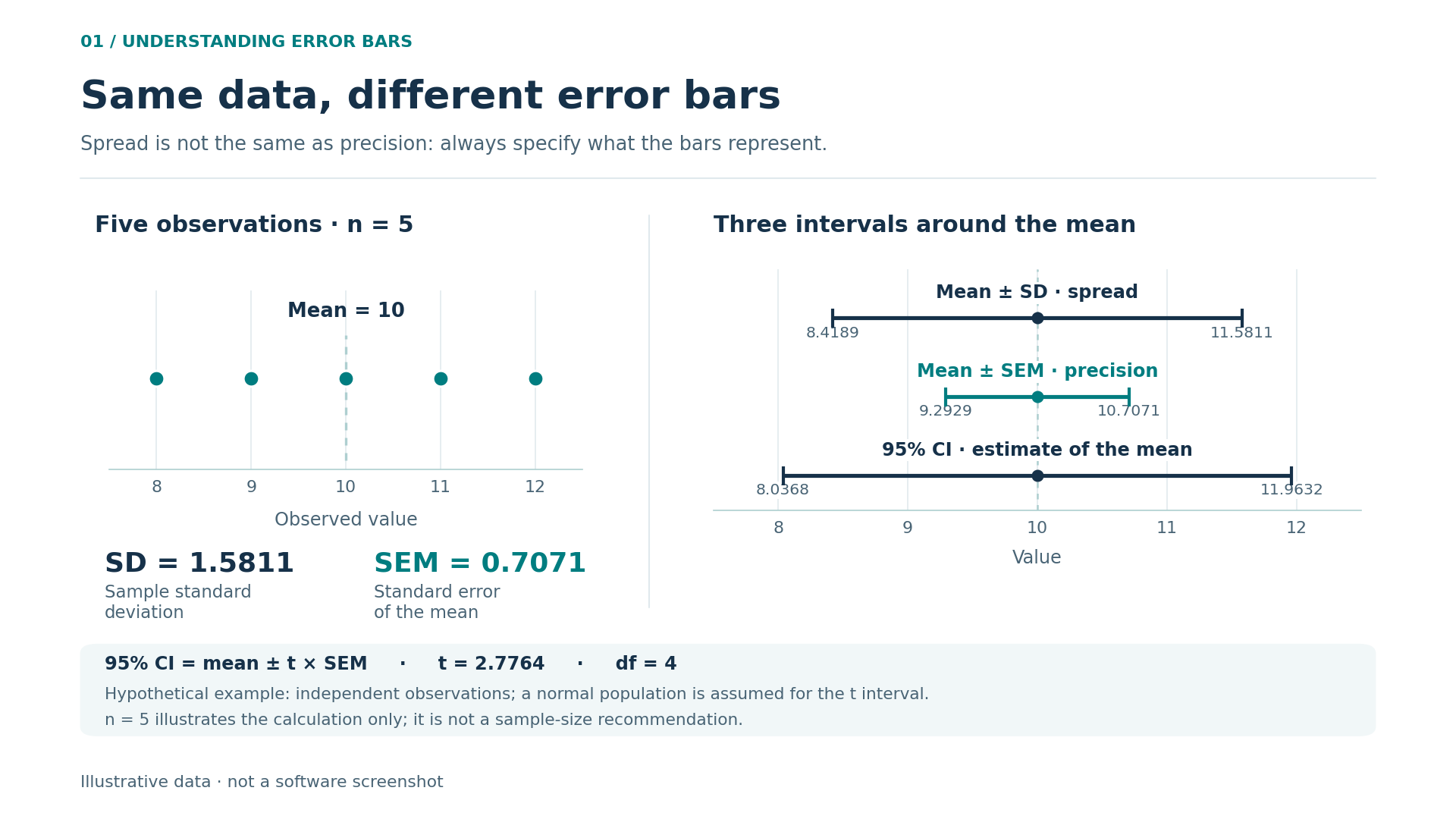
These three measures are not interchangeable. Choose the measure according to what you need the reader to understand, rather than according to which produces the shortest bars. The standard deviation, abbreviated SD, describes the spread of observations around their mean. In this example it is 1.41 MPa for each group. Use it when you want to show how much the specimens vary.
The standard error of the mean, SEM, quantifies uncertainty in the estimated mean under the sampling assumptions. It is calculated as SD divided by the square root of n. Here, 1.414 divided by the square root of six gives approximately 0.577 MPa. Being smaller than the SD does not mean the specimens are more uniform.
A 95% confidence interval adds a margin around the estimate. For a mean with an unknown population standard deviation, under the usual model of independent normal observations, the t distribution is used. With six observations, the multiplier is approximately 2.571, giving a margin of 1.484 MPa. The intervals are 8.52–11.48 MPa for A and 10.52–13.48 MPa for B.
Calculate using the available precision and round for presentation. If you replace 0.577 with 0.6 too early, small differences accumulate in the limits. Two decimal places may be enough in a figure; keep the unrounded values in the calculation file.
The interpretation of 95% concerns the procedure: if sampling were repeated many times under the same assumptions, around 95% of intervals constructed this way would contain the population mean. It does not mean that 95% of specimens lie within the interval.
7. Compare means without relying on how the graph looks
For two independent groups with a quantitative response, a t-test is one way to compare means. Welch's variant does not require equal population variances. Choose a method that fits the design and assumptions, not whichever procedure produces the smallest p-value.
In the formulation A and B example, the standard error of the difference is the square root of 2/6 + 2/6: approximately 0.816 MPa. Dividing the difference of 2 MPa by that value gives a t-statistic of 2.449. Here, the two-sided Welch test has ten degrees of freedom and gives p ≈ 0.0343. The 95% confidence interval for B minus A is approximately 0.18–3.82 MPa.
The individual intervals for A and B overlap, but the interval for the difference excludes zero. There is no contradiction: these are intervals for different parameters. That is why you should not decide whether a difference is significant solely by looking at whether the bars around two means touch. The comparison is about the difference between the means, so its uncertainty needs to be assessed for that difference.
With small samples, pay particular attention to extreme observations and whether the model is plausible. A normality test that detects no problem does not prove that the distribution is normal. In SigmaPlot, read the checks and the full report, but retain your reasoning about how the data were obtained: no wizard can reconstruct an undocumented experimental design.
8. When the data are paired
If you measure the same samples before and after treatment, the question changes. You now want to know how much each sample changes, rather than simply comparing two collections as though they were independent. The observations are paired because there is a genuine correspondence established by the design.
Arrange the columns with an identifier and both measurements. Calculate each unit's change in the same direction throughout, for example after minus before. A paired t-test analyses the mean of those changes; its normality assumption concerns the differences, and the separate pairs must be independent of one another.
A connected dot plot reveals something the means can hide: some samples improve substantially, others only slightly, and some may worsen. If one measurement is missing, do not pair the remaining observation with a different sample to complete the row. Document the missing value and the approach used in the analysis.
Having the same number of values in two columns does not make them paired. Nor is it enough that both groups were measured on the same day. Conversely, ignoring genuine pairing can waste information. If there are more time points, groups within centres or several observations per subject, the design needs an approach that represents that dependence.
9. More than two groups: ANOVA and planned comparisons
With three formulations, running a t-test for every pair seems a natural extension of the example, but it multiplies the opportunities for apparently significant results arising by chance. A one-way ANOVA first asks an overall question: whether the groups' population means are equal.
A significant overall result does not, by itself, identify which groups differ. Answering that second question requires appropriate contrasts or multiple comparisons. Comparing each formulation only with a control is not the same objective as comparing every pair. Decide which question matters before looking at the results.
Classical ANOVA makes assumptions about independence, the distribution of errors and the homogeneity of their variances. Examining residuals helps assess model fit. When the assumptions are unsuitable, consider methods for unequal variances, justified transformations or rank-based alternatives, according to the question and the tools available.
Non-parametric methods are not an automatic solution for every dataset either. They still have design requirements and do not always test the same property as a comparison of means. In your report, identify the parameter or aspect of the distribution being compared; changing the test without reviewing its interpretation may answer a different question from the original one.
10. What a p-value means, and what else to report
A p-value summarises how incompatible the data are with a null hypothesis and the model used: it gives the probability, under those conditions, of obtaining a test statistic at least as extreme as the one observed. It is not the probability that the null hypothesis is true, nor a direct measure of the effect's importance.
In the example, p ≈ 0.0343 accompanies an estimated difference of 2 MPa. If an improvement below 1 MPa has no technical value, the interval 0.18–3.82 MPa leaves that question open: it contains values both below and above the practical threshold. There is evidence of a difference within the model, but its magnitude remains imprecisely estimated.
For the same reason, p above 0.05 does not demonstrate equivalence. It may reflect a small difference, an insufficient sample or highly variable data. Demonstrating equivalence requires a relevant predefined margin and a specific procedure; a conventional comparison that is not significant is not enough.
An informative write-up would be: “In this hypothetical example, B exceeded A by 2 MPa; 95% CI for the difference: 0.18–3.82 MPa; two-sided Welch t-test, p = 0.0343; six independent specimens per group.” The reader gets the effect size, its uncertainty and the design, rather than just an asterisk.
11. Regression: examine the curve and the residuals
When the question is how a response changes with a quantitative variable, regression is more informative than artificially dividing that variable into groups. Start with a scatter plot and a model consistent with the phenomenon. For a straight line, the slope expresses the expected change in Y for each additional unit of X.
Consider another example constructed for practice: X takes the values 0, 1, 2, 3, 4 and 5; Y takes 1.2, 2.8, 4.8, 7.2, 9 and 11. The ordinary least-squares fit is estimated Y = 1 + 2X. Its residuals, observation minus prediction, are 0.2, −0.2, −0.2, 0.2, 0 and 0. R² is approximately 0.9977.
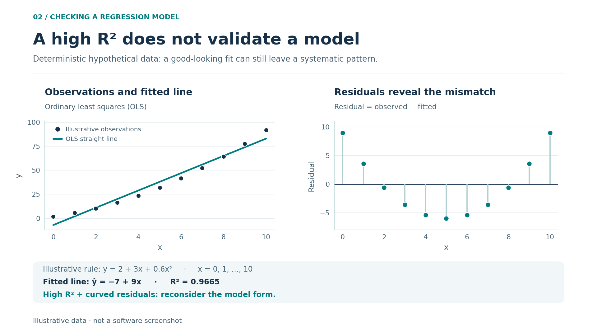
That value summarises the fit but does not replace diagnostic checks. Curvature in the residuals suggests an unsuitable functional form; a fan shape may indicate non-constant variability; a time-related sequence may reveal dependence or drift. Six points provide limited information: an apparently tidy plot does not certify that every assumption holds.
An association does not establish causation either. If temperature and response increase together, there may be a direct mechanism, a third variable or a shared time trend. Interpretation depends on the design, controls and knowledge of the process, not just the slope. Regression describes relationships; a well-designed experiment helps investigate their causes.
To see the problem, now use X = 0, 1, …, 10 and calculate Y = 2 + 3X + 0.6X². A straight-line fit achieves R² ≈ 0.9665, even though its residuals form a clear U: the data were constructed using a quadratic relationship. This shows why “high R²” does not mean “appropriate model”.
12. Non-linear fitting: do not chase the prettiest curve
A response approaching a plateau, exponential degradation or a dose–response relationship may require a non-linear model. SigmaPlot provides curve-fitting tools; Grafiti's documentation explains both the Regression Wizard and the search for initial values through dynamic fitting.
The crucial step remains choosing an equation that makes sense. Adding parameters often makes it easier for a curve to follow the points, but can produce unstable estimates and poor predictions. If you have not measured near a plateau, for example, the asymptotic value may be very poorly determined even when the curve looks convincing.
Record the equation, parameter units, initial values, constraints and any weighting. Try several reasonable starting points when the problem calls for it. Numerical convergence means the algorithm has reached a solution according to its criteria; it does not demonstrate that the solution is unique or that the model correctly describes the process.
Weighting deserves an explicit decision. If some observations have greater variance than others, giving them all equal weight may be inappropriate. Weights should reflect a defensible uncertainty model, not pull the curve towards your favourite points. Explain where the weights come from and examine the residuals consistently with that choice.
Also distinguish interpolation from extrapolation. Estimating within the measured range has a different basis from extending a curve to unobserved concentrations or times. When presenting a prediction, explain its range of validity. Do not confuse a confidence interval for the mean response with a prediction interval for a new observation: the latter includes additional variability.
13. Choose the graph that answers the question
For small groups, individual points are often more informative than a bar showing the mean. With more observations, a box plot can summarise the distribution, provided you explain what the box and whiskers represent. A histogram helps explore shape and skewness, although its appearance depends on the bin intervals chosen.
Use a scatter plot for two quantitative variables. For change over time, a line can help show the sequence, but should not suggest measurements that were never taken. In paired designs, connecting observations from the same unit makes its trajectory visible. In every case, the plot should respect how the data were collected.
Three-dimensional graphs make sense when the third dimension conveys real information. If they merely give bars depth, they add perspective and make heights harder to compare. For several experimental conditions, small panels with consistent scales may work better than a single overcrowded figure.
Before choosing a tool, think of two or three figures you regularly produce. Reviewing SigmaPlot 14 for scientific graphs and data analysis with those examples in mind helps you judge its practical usefulness: you do not need to use every option to benefit from a specialist environment.
14. Axes, error bars and legends that do not mislead
Axes are part of the argument. In a bar chart, starting the vertical axis well away from zero can exaggerate differences because we compare lengths. In a scatter plot, a restricted range may be reasonable for studying small variations, provided the scale is clear and no relevant information is hidden.
A logarithmic scale helps when positive values span several orders of magnitude or multiplicative changes matter. Label it clearly; in its usual form, it cannot accommodate zero or negative values. Changing the visual scale is not necessarily the same as transforming the variable for analysis: record those decisions separately.
Always state what the error bars show: SD, SEM, a confidence interval or another measure. If entering lower and upper limits, check whether the dialog box expects absolute limits or distances from the central value. Confusing the two formats shifts the bars even when the original numbers are correct.
Use distinguishable colours alongside different symbols or line styles. Check that the figure still makes sense in greyscale. A useful legend identifies the groups, sample size and summary shown; it need not repeat the whole methods section. Remove unnecessary decimal places, decorative backgrounds and gridlines that compete with the observations.
15. Export and preserve a reproducible analysis
Think about the destination before exporting: slides, reports and journals may require different sizes. Where the destination and your installation allow it, a vector format keeps lines and labels sharp when resized. If you need a bitmap image, set sufficient dimensions for its final display size, rather than specifying only a resolution value.
Reopen the exported file outside the program. Check special characters, units, superscripts, line thickness and any cropping. A label that seems comfortably readable on screen may become illegible when the figure is reduced to one column. Also check that the file you send reflects the latest data revision.
To repeat the work, retain the original data, prepared table, editable file, reports and final figure. Add a brief record of the software version and update, justified exclusions, transformations, test used and relevant options. For fitted models, also retain the equation and your decisions about parameters and weighting. The saved output shows what you obtained; the accompanying record explains how you obtained it and makes the steps easier to review.
An organised folder is not bureaucracy: it lets you respond to a review without reconstructing the experiment from memory. Someone receiving the project should be able to identify where each panel comes from and what changed between deliveries. Reproducibility means preserving decisions, not merely generating a similar-looking image again.
16. How to choose the right licence
Buying is simpler when you know what you need to produce. Make a short list: your usual graph types, necessary statistical tests, file-sharing requirements and the computer you will use. If you collaborate with a laboratory, check its software version and the format it needs to review results.
The Licendi offer identified for this guide is SigmaPlot 14: a perpetual licence for one PC, in English, for 64-bit Windows, with digital delivery. Language matters when following menus and documentation; the number of computers matters when planning your workstation. Check compatibility with a particular system against the requirements for that version.
“Perpetual” describes the duration of the licence offered, not a promise of new versions, compatibility with every future system or unlimited services. If you need particular installation, transfer or multi-computer arrangements, clarify them before buying rather than inferring them from the product name. This keeps your choice grounded in actual needs without confusing different licensing arrangements.
You can review the SigmaPlot 14 product page and terms at Licendi to assess that setup. The ultimate aim is not to collect features: it is to establish a clear path from data to analysis to figure. When every point, bar and conclusion has an explanation, the program becomes a practical aid to communicating your work more clearly.
17. Sources and further documentation
Official documentation consulted for general features, version distinctions and statistical principles:
- Grafiti: dedicated SigmaPlot 14.0 page and updates by version.
- Grafiti: graphing and analysis features and curve fitting and regression.
- NIST: confidence intervals for the mean and comparison of two means.
- NIST: one-way ANOVA, validation through residuals and non-linear regression.